Inland upper mantle earthquake M![]() 6.0
30km<h
6.0
30km<h![]() 80km
80km
Earthquake in the sea area
M![]() 6.5
h
6.5
h![]() 80km
80km
(M: magnitude, h: Depth of the hypocenter, same applies below)
Aftershock Probability Evaluation Methods
(1) Fundamental Concepts of the Aftershock Probability Evaluation2. Methods of Evaluating Aftershock Probability
(2) Range of the Study of Aftershock Probability Evaluation Methods
(1) Mainshock-Aftershock Pattern Clarification3. Implementation of Aftershock Probability Evaluation1) Shallow Inland Earthquakes(2) Probability Evaluation Methods Based on Statistical Models
[1] Facts Concerning 153 Independent Shallow Inland Earthquakes
[2]Methods of Judging Shallow Inland Earthquakes2)Inland Upper Mantle Earthquakes
[1]Facts Concerning 44 Independent Inland Upper Mantle Earthquakes
[2]Method of Judging Inland Upper Mantle Earthquakes3)Earthquakes in the Sea Area
[1] Facts Concerning 149 Independent Earthquakes in the Sea Area
[2] Methods of Judging Earthquakes in the Sea Area1) The Gutenberg-Richter Formula(3) Actual Application of Aftershock Stochastic Models
2) The Modified Omori Formula
3) Probability Evaluation Methods for Aftershock Activity Based on the Combination of the GR and MO Formulae
4) Application of the ETAS Model1) Average Parameters of Past Activity2) Comparison of the Past Activity and the Probability calculated from the Average Parameters
[l] Past Cases and Aftershock Occurrence Probability
[2] Past Cases and Largest Aftershock Occurrence Probability
(1) Earthquakes Whose Aftershock Probability is Evaluated4. Perspectives in the Future
(2) Aftershock Probability Evaluation Methods that Should be Implemented for the Time Being
(3)Issues that Should be Regarded to Promote Understanding of Aftershock Probability Evaluation
The Earthquake Research Committee of the Headquarters for Earthquake Research Promotion collects, organizes, and analyzes the results of surveys of earthquakes from various organizations, and carries out overall evaluations of the results of its work at regular and extra meetings in accordance with Article 7, paragraph 2, item 4 of the Special Measures Law for Earthquake Disaster Prevention.
Among evaluations of the state of earthquake activity, which is the principal responsibility of this committee, evaluations of the prospects for aftershocks following a destructive earthquake constitute a useful source of information that can be used to prevent further damage by residents and local government bodies in the region where it occurred.
The Earthquake Research Committee has been conducting concrete research on aftershock evaluation methods from the statistical and probabilistic perspectives.
This report is a summarization of the results of the committee's research.
(1) Fundamental Concepts of Aftershock Probability Evaluation
Almost every large earthquake is followed by aftershocks. And the still terrified residents of the area where a large destructive earthquake has occurred are seriously unnerved by these aftershocks.
The September 1995 Public Opinion Survey on Earthquakes (Prim Minister's Office 1995) reveals that the information which residents are most eager to obtain immediately after an earthquake are "information about the" safety of friends/relatives etc." and "seismic intensity,'' followed by "hypocenter and magnitude," ''damage to basic infrastructure and their restoration," and ''likelihood of aftershocks'' at almost equal levels of importance. And the information they want the most several hours after the earthquake is "damage to basic infrastructure and transportation facilities and prospects for their restoration,'' followed by the "likelihood of more aftershocks." "Likelihood of more aftershocks" is believed to represent their desire to know specifically when large aftershocks will occur, how large they will be, and when they will cease.
Present seismological science can not provide clear answers to all of these questions, but positive action to evaluate those aspects which can be assessed scientifically should be taken.
It is possible to use expressions of probability to evaluate aftershocks occurring in the mainshock - aftershock seismic activity pattern based on methods introduced in the following chapters. Such evaluations can make a contribution to the success of disaster protection measures in an earthquake region if, supported by a full understanding of the significance of the information, evaluations that show the residents that there is no need for needless anxiety or that they must take precautions are used to implement appropriate measures, or to minimize the damage caused the prolongation of dangerous work.
But aftershock probability is one evaluation method, and it ought to be used as part of earthquake evaluations that are now performed. So when probability information is publicly released, it should be used in an application range based on evaluations of the mainshock - aftershock Seismic activity pattern, rather than relying solely on probability.
It is also necessary that a sufficient commentary is provided and innovative measures employed to make sure that receivers of the evaluations correctly understand the numerical probability information without confusion. To guarantee this, it is essential to fix conditions for probability evaluations as needed, perform comparisons with probability in stable periods (when no earthquake has occurred), and to accompanythe evaluations with a number of past cases.
It is also necessary to continually
provide commentaries needed to disseminate knowledge concerning aftershocks
such as under what circumstances, probability evaluations are to be publicized.
This report, which summarizes aftershock probability evaluation methods for the mainshock - aftershock seismic activity pattern, considers the fact that they have been established based on present seismology.
Specifically, aftershock probability evaluation methods deal with the mainshock - aftershock seismic activity, and the aftershocks they evaluate are the so-called aftershocks in the strict sense (Note). The study whose discussions are focused on a probability evaluation method combining the modified Omori formula with the Gutenberg - Richter formula contrasts the model with past cases. The study's contents also, include items for judgments of whether a case is the mainshock - aftershock pattern, contrast the ETAS model, and a study not only of the probability of the aftershocks occurrence, but of the number of events forecasted as well.
And a study of methods of applying an aftershock probability evaluation method that accounts for the time elapsed since the mainshock is accompanied by an examination of examples of concrete expressions in evaluations.
Items related to aftershocks of great concern to residents are assumed to be the timing of large aftershocks, places where large aftershocks will occur, the shaking at specified locations that a large aftershock will cause, and so on. Some study of these issues has been carried out, but because under present circumstances, it is thought that an evaluation method good enough to permit the public release of its results has not been established, the results of this study are not reported.
Note) When an earthquake has occurred,
it is generally followed by a number of earthquakes smaller than the first
earthquake at locations close to the location of the first earthquake.
The first earthquake is called the mainshock and the smaller earthquakes
that follow it are called the aftershocks, and this seismic activity pattern
is called the mainshock - aftershock pattern. And the aftershock distribution
immediately after the mainshock (from a Few hours to a day) almost always
represents the focal region of the mainshock. An aftershock in the strict
sense refers to these nearby aftershocks, while those occurring tar from
that region are referred to as so-called aftershocks in the wide sense
or else they are called induced earthquakes. The term for a relatively
small earthquake in the focal region of a mainshock prior to the mainshock
is foreshock.
(1) Mainshock - Aftershock Pattern Clarification
The aftershock probability evaluation method is an effective way to evaluate aftershock activity of the mainshock - aftershock pattern. In order to move efficiently to the aftershock probability evaluation described below, this section explains a method of empirically clarifying whether activity is the mainshock - aftershock pattern at earliest stage of earthquake activity based on examples of past earthquakes (Ito et a1. 1999).
For convenience, the following categorization is done with reference to the magnitude and hypocenter of the first earthquake.
shallow inland earthquake MA series of seismic activities close both spatially and tempora11y to the first earthquake is treated as a single independent case (Hoshiba et a1, 1993). The range of ''inland" is shown in Fig. 1. "Sea area'' indicates locations outside the range of "inland".5.5 h
30km
Inland upper mantle earthquake M
Earthquake in the sea area M
(M: magnitude, h: Depth of the hypocenter, same applies below)
[1] Facts Concerning 153 Independent Shallow Inland Earthquakes
( M![]() 5.5,
h
5.5,
h![]() 30km,
1926-1995, Fig.1.).
30km,
1926-1995, Fig.1.).
a) Case of M![]() 6.4
Earthquakes
6.4
Earthquakes
No earthquake greater than this occurred later.
b) Case of 6.3![]() M
M![]() 6.0
Earthquakes
6.0
Earthquakes
- In one case, a larger earthquake occurred.
December 26, 1949: An M6.4 earthquake occurred 7 minutes after an M6.3 earthquake (Imaichi Earthquake).
- In two cases, equally large earthquakes
occurred.
Fig.1. Shallow Inland Earthquakes
M![]() 5.5,
h
5.5,
h![]() 30km,1926 to
1995
30km,1926 to
1995
The circles indicate areas within
20 km of a Quaternary volcano. The polygon surrounding the Japanese Archipelago
encloses the "inland" areas.
Fig.2. Shallow Inland Earthquakes
(Mf-Ml![]() 0.3)
0.3)
The circles indicate areas within
20 km of a Quaternary volcano.
Table 1-1 Seismic Activity With A
Small Difference Between the Magnitude of the First earthquake Mf
and the Magnitude of the Largest Subsequent Earthquake M1 (Mf-Ml![]() 0.3)
0.3)
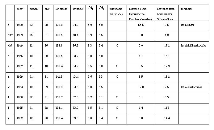
Table 1-2 Seismic Activity With A
Small Difference Between the Magnitude of the First earthquake Mf
and the Magnitude of the Largest Subsequent Earthquake M1 (Mf-Ml![]() 0.3)
0.3)
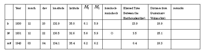
Table 1-3 Seismic Activity With A
Small Difference Between the Magnitude of the First earthquake Mf
and the Magnitude of the Largest Subsequent Earthquake M1 (Mf-Ml![]() 0.3)
0.3)
March 4, 1943: An M6.2 earthquake occurred 0.4 days after an M6.2 earthquake (Tottori).
December 22, 1956: An M6.0 earthquake occurred 1.13 days after an M6.0 earthquake (Miyake-jima).
c) Case of M![]() 5.5 Earthquakes
5.5 Earthquakes
Approximately 50% of M ![]() 5.5 earthquakes (76 of the 153 cases) occurred within 30 km of a Quaternary
volcano (note: volcanoes active in recent geological ages or still active
) (Seino et a1, 1995). About 17% of these (13 of 76 cases, see Tables 1-1,
2, and Fig. 2) were earthquakes of similar magnitude(Mf-M1
5.5 earthquakes (76 of the 153 cases) occurred within 30 km of a Quaternary
volcano (note: volcanoes active in recent geological ages or still active
) (Seino et a1, 1995). About 17% of these (13 of 76 cases, see Tables 1-1,
2, and Fig. 2) were earthquakes of similar magnitude(Mf-M1![]() 0.3 : Mf is the M of the first earthquake
Ml
is the largest M of the followed earthquakes : Cases where M1
> Mf are included. Same applies below), which is significantly
higher than the 5% (4/77; Table 1-3 and Fig. 2) in other regions (the hypothesis
that the probabilities in each region are the same can be rejected at a
significance level of 1%). This means that within 30 km of a Quaternary
volcano, an earthquake of similar magnitude is likely to occur. There were
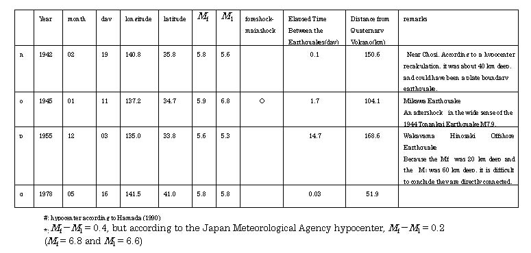
8 cases of the foreshock - mainshock pattern seismic activity that is a
concern of this study, and about 75% of the activity is within 20 km of
a Quaternary volcano (6/8 cases: Table 1-1). Even in regions further than
20 km from a Quaternary volcano, two were foreshock - mainshock pattern
( l: the earthquake near Kumamoto and o: Mikawa Earthquake, see Tables
1-2,3).
0.3 : Mf is the M of the first earthquake
Ml
is the largest M of the followed earthquakes : Cases where M1
> Mf are included. Same applies below), which is significantly
higher than the 5% (4/77; Table 1-3 and Fig. 2) in other regions (the hypothesis
that the probabilities in each region are the same can be rejected at a
significance level of 1%). This means that within 30 km of a Quaternary
volcano, an earthquake of similar magnitude is likely to occur. There were
8 cases of the foreshock - mainshock pattern seismic activity that is a
concern of this study, and about 75% of the activity is within 20 km of
a Quaternary volcano (6/8 cases: Table 1-1). Even in regions further than
20 km from a Quaternary volcano, two were foreshock - mainshock pattern
( l: the earthquake near Kumamoto and o: Mikawa Earthquake, see Tables
1-2,3).
Note: Quaternary volcanoes were revised based on Volcanoes of Japan (First edition: Isshiki et al., 1968a, Second edition: Ono et al.,1981), and for the Hokkaido region, the results of a correction by Nakagawa et al. (1995) were incorporated. The latitude and longitude of each volcano is based on the Selected Literatures on Volcanoes (First edition: Isshiki et al., 1968b) and the General Survey of Active Volcanoes in Japan (Japan Meteorological Agency, second edition: 1996) and on Otani et al.(1993). Future measurements of the age of rocks may result in a revision of the list of volcanoes classified as Quaternary volcanoes.
[2] Methods of Judging Shallow Inland Earthquakes
- If an earthquake magnitude is
M![]() 6.4,
it is treated as a mainshock.
6.4,
it is treated as a mainshock.
- If an earthquake magnitude is
6.3![]() M
M![]() 5.5
and it is further than 20km from a Quaternary volcano, it is treated as
a mainshock. But when these plural earthquakes occurred, or when an oceanic
magnitude M8 class earthquake occurred under the ocean nearby within
the past 2 or 3 years, it could be a foreshock.
5.5
and it is further than 20km from a Quaternary volcano, it is treated as
a mainshock. But when these plural earthquakes occurred, or when an oceanic
magnitude M8 class earthquake occurred under the ocean nearby within
the past 2 or 3 years, it could be a foreshock.
- If an earthquake with magnitude
6.3![]() M
M![]() 5.5
occurs within 30 km of a Quaternary volcano, there is a high likelihood
of an earthquake almost as large as the first earthquake occurring. And
within 20 km of a Quaternary volcano, it could be a foreshock.
5.5
occurs within 30 km of a Quaternary volcano, there is a high likelihood
of an earthquake almost as large as the first earthquake occurring. And
within 20 km of a Quaternary volcano, it could be a foreshock.
[1] Facts Concerning 44 Independent Inland Upper Mantle Earthquakes
(M![]() 6.0,30km<h
6.0,30km<h![]() 80km, 1926 to 1995: Fig. 3)
80km, 1926 to 1995: Fig. 3)
1) No subsequent earthquake larger than the first earthquake occurred.
2) Earthquakes of approximate magnitude
(Mf-M1![]() 0.3) occurred only once (1/44 = 2%) (Table 2. Fig. 3.).
0.3) occurred only once (1/44 = 2%) (Table 2. Fig. 3.).
[2]Method of Judging Inland Upper Mantle Earthquakes
- If the magnitude M![]() 6.0, it is treated as the mainshock.
6.0, it is treated as the mainshock.
Table 2. Seismic Activity With a
Small Difference Between the Magnitude of the First Earthquake Mf
and the Magnitude of the Largest Subsequent Earthquake M1(Mf-M1![]() 0.3)
0.3)
(Inland Upper Mantle Earthquakes)
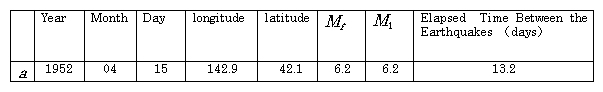
Fig. 3. Inland Upper Mantle Earthquakes
M![]() 6.0,
30 km < h
6.0,
30 km < h![]() 80km, 1926 to 1995
80km, 1926 to 1995
The polygon enclosing the Japanese
Archipelago indicates the range of ''inland.''
[1] Facts Concerning 149 Independent
Earthquakes in the Sea Area(M ![]() 6.5,h
6.5,h![]() 80km, 1926 to 1995: Fig. 4)
80km, 1926 to 1995: Fig. 4)
a)Case of M![]() 7.0 Earthquakes
7.0 Earthquakes
There are only one case in which
an M![]() 7.0 earthquake
was followed by a larger earthquake. Foreshocks of M6.5, 6.6, 6.7,
and 7.0 occurred during the three day period prior to the Etorofu Island
Offshore Earthquake (M 7.3) of March 25, 1978
7.0 earthquake
was followed by a larger earthquake. Foreshocks of M6.5, 6.6, 6.7,
and 7.0 occurred during the three day period prior to the Etorofu Island
Offshore Earthquake (M 7.3) of March 25, 1978
b)Case of M![]() 6.5
Earthquakes
6.5
Earthquakes
Earthquakes of approximate magnitude
(Mf-M1![]() 0.3) in 18 cases (18/149 = 12%) (Table 3 and Fig. 5).
0.3) in 18 cases (18/149 = 12%) (Table 3 and Fig. 5).
Regions where an oceanic earthquake
is likely to be followed by a subsequent earthquake of similar magnitude
(sequential occurrence regions)-part of the sea bottom offshore from Sanriku
or Eterofu Island for example-were experientia11y clarified and are presented
in Fig. 5. Approximately 31% (46/149 cases) of M![]() 6.5
earthquakes occurred in the sequential occurrence regions, as did about
67% (12/18 cases) of the earthquakes of similar magnitude (Mf-M1
6.5
earthquakes occurred in the sequential occurrence regions, as did about
67% (12/18 cases) of the earthquakes of similar magnitude (Mf-M1![]() 0.3) (Table 3-1, Fig. 5). The 26%(12/46 cases) of earthquakes of similar
magnitude occurring in the sequential occurrence regions is significantly
higher than the 6% (6/103 cases: Table 3-2) of such earthquakes occurring
outside of these regions (the hypothesis that the probabilities are identical
in each region can be rejected at a significance level of less than 1%).
And the foreshock - mainshock pattern occurred at a rate of 9% (4/46 cases)
in the sequential occurrence regions, while in other regions the magnitude
of all subsequent earthquakes was smaller, so that these are viewed as
the mainshock - aftershock pattern.
0.3) (Table 3-1, Fig. 5). The 26%(12/46 cases) of earthquakes of similar
magnitude occurring in the sequential occurrence regions is significantly
higher than the 6% (6/103 cases: Table 3-2) of such earthquakes occurring
outside of these regions (the hypothesis that the probabilities are identical
in each region can be rejected at a significance level of less than 1%).
And the foreshock - mainshock pattern occurred at a rate of 9% (4/46 cases)
in the sequential occurrence regions, while in other regions the magnitude
of all subsequent earthquakes was smaller, so that these are viewed as
the mainshock - aftershock pattern.
[2] Methods of Judging Earthquakes
in the Sea Area (M![]() 6.5,
h
6.5,
h![]() 80
km)
80
km)
- If it is an M![]() 7.0 earthquake, it is treated as a mainshock.
7.0 earthquake, it is treated as a mainshock.
- If it is a 6.9![]() M
M![]() 6.5
earthquake and it is not in the sequential occurrence regions, it is treated
as a mainshock.
6.5
earthquake and it is not in the sequential occurrence regions, it is treated
as a mainshock.
- If a number of 6.9![]() M
M![]() 6.5
earthquakes occur in the sequential occurrence regions, and their magnitude
gradually increases, they may be foreshocks.
6.5
earthquakes occur in the sequential occurrence regions, and their magnitude
gradually increases, they may be foreshocks.
Table 3-1 Seismic Activity With a
Small Difference Between the Magnitude of the First Earthquake Mf
and
the Magnitude of the Largest Subsequent Earthquake M1(Mf-Ml![]() 0.3) (Earthquakes in the Sea Area)
0.3) (Earthquakes in the Sea Area)
Table 3-2 Seismic Activity With a
Small Difference Between the Magnitude of the First Earthquake Mf
and
the Magnitude of the Largest Subsequent Earthquake M1(Mf-M1![]() 0.3) (Earthquakes in the Sea Area)
0.3) (Earthquakes in the Sea Area)
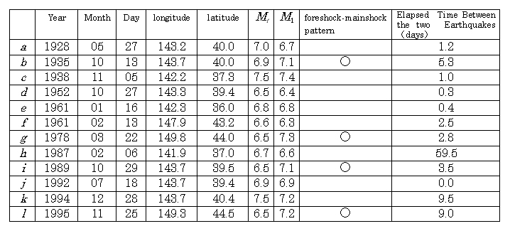
Fig. 4. Earthquakes in the Sea Area
M![]() 6.5,
h
6.5,
h![]() 80
km, 1926 to 1995
80
km, 1926 to 1995
The polygons around the Sanriku offshore
region and the Etorofu Island offshore region enclose sequential occurrence
regions.
Fig. 5. Earthquakes in the Sea Area
and Sequential Occurrence Regions (Mf-M1![]() 0.3)
0.3)
The polygons around the Sanriku offshore
region and the Etorofu Island offshore region enclose the sequential occurrence
regions.
A model that clarifies the nature of aftershock activity and a model that clarifies the relationship between the number of shocks and M by statistical processing of the past seismic activity of the mainshock - aftershock pattern have been reported. In section (2), these statistical models and aftershock probability evaluation methods devised by combining them are described.
The modified Omori- Formula and the ETAS (Epidemic Type Aftershock Sequence) model have been technically established as methods of clarifying aftershocks.
The ETAS model can be used not only to evaluate aftershock activity; but also to appropriately evaluate background seismic activity, and it can also be used to evaluate earthquake swarms. In this sense, it can be called an extension of the modified Omori Formula, but the M values of the aftershocks are necessary. So a method based on the modified Omori Formula will be studied first, then in part 4), the application of the ETAS model will be described.
An aftershock probability evaluation
as it is used here refers to stochastically expressing and evaluating the
frequency that an aftershock of a certain magnitude will occur. The modified
Omori Formula forecasts the number of aftershocks that will occur, but
in order to perform a probability evaluation that accounts for the magnitude
of the aftershocks, it is necessary to combine this formula with the Gutenberg
- Richter Formula.
It is known that large aftershocks do not occur frequently.
Quantitatively, the larger the magnitude
of aftershocks, their number declines exponentially. This empirical rule
is called the Gutenberg- Richter's relationship (Gutenberg and Richter,
1941). If, expressed in the form of a mathematical expression, the frequency
of aftershocks between M and M+dM is denoted to be
n(M)
dM:
![]()
Or
![]()
"log" above represents the common
logarithm. This formula is called the Gutenberg-Richter Formula below referred
to as the ''GR Formula''). a and b are constants. a
is the parameter that expresses the level of overall aftershock activity.
b is a value that is closely related to the number of small aftershock
/ the number of large aftershock ratio, and its large value means that
the number of large earthquakes is relatively small. If a graph is plotted
from formula (1) with the magnitude M represented by the X
axis and log n(M) by the Y axis, it is a straight
line with the Y section of the line corresponding to a and the incline
corresponding to b.
N(M), the total cumulative number of aftershocks larger than M, which
is represented as:
is also used in place of n(M)
.
Using equation(2), equation (3) is
expressed as:
Here, ![]() =
b ln10, and'ln'
is the natural logarithm.
=
b ln10, and'ln'
is the natural logarithm.
Taking the common logarithms on both
sides of equation (4) and ![]() ,
the following equation is obtained.
,
the following equation is obtained.

In the case of actual observation,
as the magnitude M declines, it becomes difficult to detect earthquakes.
If the lower detection limit of this M is assumed to be Mth:
is obtained, and (M- Mth)
is shown to be exponential distribution. To translate this to the probability
density function, it is Sufficient to assume that:
![]()
in order that when n(M)
has been integrated from M to ![]() for
M, it is standardized as 1. It is possible to state that equation
(7) is obtained by standardizing equation (2), and a that indicates the
level of overall aftershock activity is not included.
for
M, it is standardized as 1. It is possible to state that equation
(7) is obtained by standardizing equation (2), and a that indicates the
level of overall aftershock activity is not included.
Aftershock activity declines monotonously
over time. Quantitatively, the number of aftershocks per unit of time![]() is, with K, c, and p as parameters, represented by:
is, with K, c, and p as parameters, represented by:

Here, t is the elapsed time
with its origin point the occurrence of the mainshock. Equation (8) is
called the modified Omori Formula (Utsu 1957, Utsu 196l, below called the
"MO Formula"). When p = 1, it is simply called the Omori Formula
(Omori, 1894). p, which represents the degree of the damping over
time, is normally either 1 or a slightly larger value. The role of c
is to appropriately round off complex aspects immediately after the mainshock,
and it is normally less than 0.1 days.
K is proportional to the total
number of aftershocks when p and c are constant. Because the total
number is widely scattered according to each activity, and is also dependent
on Mth, if for example, it is assumed that:
![]()
for differing activity, it is necessary
to compare logKM3 etc. If a graph of equation(8) is plotted
with log t as the X axis and logν as the Y axis,
it becomes a straight line after a sufficient amount of time has elapsed
following the mainshock (t >>c), the incline of this straight line
corresponds to-p, and the X section corresponds almost exactly
with (logK)/p.
If attention is focused only on the
times that aftershocks occur and the time elapsed from the mainshock is
represented by the horizontal axis and the total cumulative earthquake
frequency by the vertical axis, a stepped graph is obtained. The way that
aftershocks occur is determined only by the mainshock that is overwhelmingly
large, which means that if it is hypothesized that the next aftershock
is not dependent on the way the previous aftershock occurred, the occurrences
of aftershocks follow a non-stationary Poisson process. In this case, it
is possible to interpret the MO Formula as the aftershock probability by
setting a sufficiently small unit time. If this is represented by a formula,
the probability![]() of
an aftershock occurring between time t and time t+dt
is represented as:
of
an aftershock occurring between time t and time t+dt
is represented as:

And in order to find K, p,
and c for actual aftershock activity, the maximum likelihood method
is used. In this case, the logarithmic likelihood function ln L
is obtained from the following equation (Ogata, 1983), and it can be estimated
by finding the values of K, p, and c that maximize
this (maximum likelihood estimate).
Here, N is the number of
aftershocks observed during the time elapsed since the mainshock Tl
to
T2
, and ti ( i =1,2,---,N) represent the times
when each aftershock occurs. And A( Tl
to
T2
) is 1/K of the time integral of the MO Formula.
It is possible to evaluate the probability
of aftershock activity by combining the GR Formula with the MO Formula.
If it is assumed that the magnitudes M of aftershocks occurring between
time t and t+dt are distributed in accordance with
the GR Formula, the probability![]() of
earthquakes whose magnitude is between M and M+dM
occurring between t and t+dt is, using equation (7),
obtained as shown below.
of
earthquakes whose magnitude is between M and M+dM
occurring between t and t+dt is, using equation (7),
obtained as shown below.
The probability ![]() of an aftershock with magnitude greater than M occurring between
times t and t+dt is, by integrating equation (13)
for the magnitude from M to
of an aftershock with magnitude greater than M occurring between
times t and t+dt is, by integrating equation (13)
for the magnitude from M to![]() ,
obtained as shown below.
,
obtained as shown below.
Taking advantage of the fact that
the expected value of the Poisson distribution of index ![]() is
is ![]() , the expected
value of the frequency
N(Tl ,T2)
the number of events forecasted of earthquakes larger than M during
the time from Tl
to T2
is, using the
time integral (12) of the MO Formula, obtained by:
, the expected
value of the frequency
N(Tl ,T2)
the number of events forecasted of earthquakes larger than M during
the time from Tl
to T2
is, using the
time integral (12) of the MO Formula, obtained by:
The probability Q of one
or more aftershock of M or greater occurring since the mainshock,
in the time Tl to T2 is, using the
Poisson distribution formula, found by:
Equation (15) is the formula that
calculates the number of aftershocks forecasted and equation (16) is the
formula for the aftershock occurrence probability.
The significance of the variables is explained. K, p, and c, the parameters of the MO Formula that defines the special characteristics of the aftershock activity, are determined to provide the best explanation of actual aftershock activity. K is approximately proportional to the total number of aftershocks. p represents the extent of time damping. c compensates for complex aspects immediately after the mainshock.
![]() represents the relationship of
b and
represents the relationship of
b and ![]() =
b
ln 10
=
b
ln 10 ![]() 2.30b
in the GR formula. b is a value that is closely related to the number
of small aftershocks/ that of large aftershocks ratio, and its large value
indicates relatively small number of deal with in large earthquakes. Mth,
the magnitude of the smallest earthquake processed using the MO Formula
or the GR Formula. It is premised that all aftershocks larger than Mth
are observed without omissions.
Tl
to T2
, Which represent the beginning and the end of the period during which
the aftershock probability is evaluated, both represent elapsed time following
the mainshock. A (Tl ,T2) is provided
by equation (12). It must be kept in mind that equation (16) does not represent
the probability of an aftershock that matches conditions occurring exactly
once; it represents the probability of it occurring more than 1 time.
2.30b
in the GR formula. b is a value that is closely related to the number
of small aftershocks/ that of large aftershocks ratio, and its large value
indicates relatively small number of deal with in large earthquakes. Mth,
the magnitude of the smallest earthquake processed using the MO Formula
or the GR Formula. It is premised that all aftershocks larger than Mth
are observed without omissions.
Tl
to T2
, Which represent the beginning and the end of the period during which
the aftershock probability is evaluated, both represent elapsed time following
the mainshock. A (Tl ,T2) is provided
by equation (12). It must be kept in mind that equation (16) does not represent
the probability of an aftershock that matches conditions occurring exactly
once; it represents the probability of it occurring more than 1 time.
Real earthquake activity can not be represented solely as mainshock - after shock pattern,. it involves complex and diverse phenomena such as earthquake swarms, secondary aftershocks, and relations with other regions.
The ETAS model, which is considered a superior approximation and is based on the concept that every earthquake is accompanied by some degree of aftershock activity, is an effective tool for the analysis of seismic activity in a specific region or of long term seismic activity (Ogata 1986, 1988, 1989, 1992, 1994).
To clarify aftershock activity in the strict sense, it is particularly important to grasp the level of aftershock activity following a secondary aftershock and determine whether or not aftershocks is smoothly decreasing. It can be thought of as an expansion model that clarifies the activity accompanying a secondary aftershock using the MO Formula by superimposing the aftershock activity of the mainshock and the activity of two or three series of secondary aftershocks at the most. Analysis to clarify whether the secondary aftershock activity is or is not significant and whether the p value differs or not can be done by using Akaike information criterion (Akaike, 1974) to compare the degree of conformity of these differing models (Ogata 1983, Ogata and Shimazaki 1984, Matsu'ura 1986, Utsu et al, 1995).
But when the activity is more complex, and particularly when performing analysis to determine whether or not aftershocks are smoothly decreasing, with methods based on the simple MO Formula or the expanded model explained above, depending on which period is being analyzed, the forecast probability fluctuates according to circumstances, making it difficult to obtain objective conclusions. Using the ETAS model, it is possible to objectively determine whether or not the aftershock activity has fluctuated at a particular time.
It is not clear, however, just What
the quiescence in the aftershock activity demonstrated by these analysis
methods actually represents, and it is important to gather more cases to
contribute to continued research on ways to evaluate aftershock activity
of this kind.
The actual application of the probability
evaluation methods based on the statistical models described in Part (2)
involves the problem of determining whether it is or is not possible to
stably find the parameters (K, c, p, b) for aftershock activity
immediately following a mainshock. If the average parameters for the aftershock
activity are known, there is a possibility that these this can be used
effectively as preliminary data until the actual data is available. For
this reason, specific parameters for the aftershock stochastic model combining
the GR Formula and the MO Formula (below referred to as "aftershock stochastic
model") or past cases are compared, and their application range is studied.
The values of average parameters of the aftershock stochastic model of past seismic activity are based on the following sources. Because K is dependent on the lower detection limit Mth and the values that make the Mth uniform are widely scattered for each activity, the average values are not listed here.
Table 4. Aftershock Parameters for
Earthquakes Near Japan (median Values)
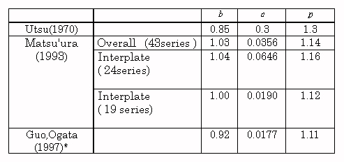
* The median values of c
and
p of the ETAS model were used.
Table 4 shows that values obtained
from recent analysis results are approximately 1.0 for b, between
0.02 and 0.06 for c, and about 1.1 for p. Because the MO
Formula parameters are not found independently, there is a tradeoff between
each of the parameters during analysis. If it is hypothesized that c
and p are the average parameters ,![]() and
and ![]() , it is
possible to compare the average parameters (K, c, p) separately
with the parameters (K,
, it is
possible to compare the average parameters (K, c, p) separately
with the parameters (K, ![]() ,
, ![]() )
to judge which is appropriate. Specifically, by comparing AIC of each of
the models:
)
to judge which is appropriate. Specifically, by comparing AIC of each of
the models:

the model with the smaller AIC can
be used. The documents cited in Table 4 do not include studies of this
kind. And many of the earthquakes analyzed in Table 4 were accompanied
by a few aftershocks. This is a result of the fact that the hypocenters
were far away or that the data was obtained at a time when earthquake detection
capability was poor. An average image comprehensively analyzed concerning
the level of aftershock activity is not obtained from these sources. This
substantial scattering may be a property of natural phenomena, but obtaining
an average image is important, because it permits information about average
aftershock activity to be obtained from these parameters. This information
includes the magnitude of the largest aftershock relative to the M of
the mainshock below, ''M0"), or in which period after
the mainshock the largest aftershock often occurs; information to be used
to consider planning for protection from aftershocks, and through a comparison
with it, to objectively evaluate the level of the aftershock activity.
To find this average image, it is necessary to collect cases Studied based on the regional categorization outlined in Part (1) and the earthquake category (interplate, intraplate, etc.) and at the same time, to comprehensively consider aftershock activities from high level to low level in order to determine if it is possible to perform a categorization of this activity. The following sections [1] to [3] introduce specific study methods.
[1]Method Based on the Value of K
It is possible to compare differing aftershock activities using logKM3 (value obtained by correcting the value K of the activity by a certain threshold value) defined by equation (9), and it is also possible to contribute to the evaluation of aftershock probability by surveying the relationship between this value and M0.
[2] Method Based on the Aftershock Activity Standardization Parameters
Because K in the MO Formula
depends on the values Mth, M0 and b
of aftershock activity, the following standardization is considered. In
brief, aftershock activity is characterized by:

(Utsu 1970, Reasenberg and Jones
1989, 1994, Abe 1991, 1994, Matsu'ura 1993, Shizuoka Prefecture Earthquake
Measures Section, 1993). From this:
is obtained, and using this relationship,
equation (16) can be expressed as:

[3] Method Based on the Difference
Between M of the Mainshock and M of the Largest Aftershock
Aftershocks generally conform to
the GR Formula, but mainshock magnitude M0 is often far
greater than the GR Formula (Utsu, 1957). An investigation of the difference
D
(= M0-Mm) between the mainshock
M0
and
the largest aftershock Mm (same applies below) can contribute
to an aftershock probability evaluation. Specifically, it is based on the
following procedure. First, based on the MO Formula, the forecast number
of earthquakes of M![]() Mth
during time from 0 to
Mth
during time from 0 to ![]() is
estimated to be KA(0,
is
estimated to be KA(0, ![]() )
for M = Mth in equation (15). While the number
of aftershocks for the same time period forecasted by using the GR Formula
is estimated to be Nth (0 ,
)
for M = Mth in equation (15). While the number
of aftershocks for the same time period forecasted by using the GR Formula
is estimated to be Nth (0 ,![]() ).
Equalizing these, we obtain:
).
Equalizing these, we obtain:

![]() is the period of time until the aftershock activity ends, but because Nth
(0 ,
is the period of time until the aftershock activity ends, but because Nth
(0 ,![]() ) diverges
when p
) diverges
when p![]() 1.0,
1.0,![]() must be substituted by taking a sufficiently large value.
must be substituted by taking a sufficiently large value.
From equation (20):
Using this, equation (16) can be
expressed as:
The method presented in [2] above,
where ![]() is
not dependent on the mainshock
M0 , is based on an idea
to find the difference among earthquakes with different types in different
regions. The value of D is provided as 1.4 as an average by Utsu
(1957), and afterwards, based on its relationship with
M0
, Utsu (1969) found:
is
not dependent on the mainshock
M0 , is based on an idea
to find the difference among earthquakes with different types in different
regions. The value of D is provided as 1.4 as an average by Utsu
(1957), and afterwards, based on its relationship with
M0
, Utsu (1969) found:
![]()
D in this equation decreases
as M0 increases; It suggests that the level of aftershock
activity relative to the magnitude of the mainshock can increase as the
value of M0 increases. Equation (23) is based on the
belief that even earthquakes which are not followed by observed aftershocks
are in fact followed by undetectable aftershocks. Therefore, and it is
necessary to distinguish cases dealing only with earthquakes whose aftershocks
can be observed.
Problems with the method introduced
in [3] include the extremely large scattering of the value of D
and the fact that when p![]() 1.0,
it is necessary to know what value should be taken instead of
1.0,
it is necessary to know what value should be taken instead of ![]() to calculate A(0,
to calculate A(0,![]() ).
).
When actually performing calculations
of this activity, it is acceptable to survey the time period in which the
aftershocks caused by mainshock M0 are below the level
of the background seismic activity and use values in accordance with the
results of this survey. In order to consider an index of the level of aftershock
activity that is not dependent upon D, it is assumed that:
and substituting this in equation
(21) obtains:
The largest aftershock Mm
can be estimated based on:
from the relationship in equation
(20). Using this relationship, equation (16) can be expressed as:

By surveying the relationship of
D
and ![]() with the
characteristics of the region or with the earthquake classification as
a way of expanding the method introduced in [3], it is possible to contribute
to aftershock probability evaluations.
with the
characteristics of the region or with the earthquake classification as
a way of expanding the method introduced in [3], it is possible to contribute
to aftershock probability evaluations.
In addition to these methods above,
it is necessary to compare other methods, for example, to survey the characteristics
of the region using that numbers of aftershocks follow negative binomial
distribution (Okada, 1979).
Probability calculated based on the methods presented in Part 1) do not provide exactly the same numerical results. Here these are compared with past cases.
[1] Past Cases and Aftershock Occurrence Probability
The average parameters to be applied to the aftershock stochastic model are established as explained below.
Trial calculation parameter ![]() :
The parameter D that represents the level of aftershock activity
with method [3] is used.
:
The parameter D that represents the level of aftershock activity
with method [3] is used. ![]() ,
, ![]() and
and ![]() applied are the medians for all the cases in and around Japan (Matsu'ura,1993).
And the probability of an aftershock greater than M5.0 occurring
once or more following an M6.0 mainshock assuming
applied are the medians for all the cases in and around Japan (Matsu'ura,1993).
And the probability of an aftershock greater than M5.0 occurring
once or more following an M6.0 mainshock assuming ![]() =
1.2 (
=
1.2 (![]() )
and the probability of an aftershock greater than M6.0 occurring
once or more following an M7.0 mainshock assuming that
)
and the probability of an aftershock greater than M6.0 occurring
once or more following an M7.0 mainshock assuming that ![]() =
1.1 (
=
1.1 (![]() ) are Separately
calculated on trial.
) are Separately
calculated on trial.
Trial calculation parameter ![]() :
Method [2] is used, and the median value for cases of intraplate earthquakes
(
:
Method [2] is used, and the median value for cases of intraplate earthquakes
( ![]() -2.36:
-2.36:![]() )
of Matsu'ura (1993) is applied to trial calculation of the probability
of an aftershock greater than M5.0 ccurring once or more following
an M6.0 mainshock, and the median value for cases of interplate
earthquakes (
)
of Matsu'ura (1993) is applied to trial calculation of the probability
of an aftershock greater than M5.0 ccurring once or more following
an M6.0 mainshock, and the median value for cases of interplate
earthquakes ( ![]() -2.36:
-2.36:![]() )
is applied to trial calculation of the probability of an aftershock greater
than M6.0 occurring once or more following an M7.0 mainshock.
)
is applied to trial calculation of the probability of an aftershock greater
than M6.0 occurring once or more following an M7.0 mainshock.
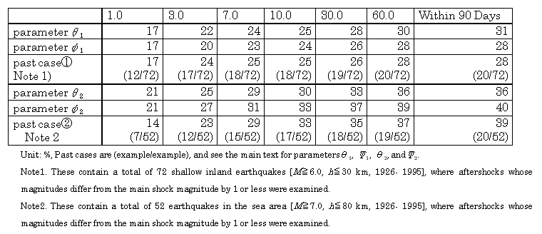
Trial calculations using these parameter and setting T1= 0, T2= 1, 3, 7, 10, 30, 60, 90 (days), were compared with past cases (shallow inland earthquakes, earthquakes in the sea area) (Table 5-1).
The past cases presented in Table 5-1 can not,
strictly speaking, be compared considering the relationship between a mainshock
M0
and aftershock activity expressed by formula (23), but the overa11 tendencies
of the probability based on the trial calculation Parameter conform with
those of the past cases. ![]() for the trial calculation
for the trial calculation ![]() is a value that is close to the average of the past activities of different
magnitude M . The results of the trial calculations for
various types of earthquake based on trial calculation
is a value that is close to the average of the past activities of different
magnitude M . The results of the trial calculations for
various types of earthquake based on trial calculation ![]() are
also close to the past cases. It is not possible from this to determine
if there is a regional difference between earthquakes in the sea area and
shallow inland earthquakes or a difference in the mainshock
M0.
The important fact is that it is possible to represent probability almost
identical to that seen in past cases using the average parameters
are
also close to the past cases. It is not possible from this to determine
if there is a regional difference between earthquakes in the sea area and
shallow inland earthquakes or a difference in the mainshock
M0.
The important fact is that it is possible to represent probability almost
identical to that seen in past cases using the average parameters ![]() ,
, ![]() and
and ![]() for
the aftershock stochastic model.
for
the aftershock stochastic model.
A comparison of the two trial calculations![]() and
and ![]() reveals
that value
reveals
that value ![]() =
1.2 in trial calculation
=
1.2 in trial calculation ![]() is itself a parameter that signifies activity of the largest aftershock
Mm
= 4.8 following a mainshock M0 = 6.0, and when the probability
of a relatively large aftershock is calculated, a slightly larger value
is obtained with the trial calculationΨ (method [2]) than with the trial
calculation
is itself a parameter that signifies activity of the largest aftershock
Mm
= 4.8 following a mainshock M0 = 6.0, and when the probability
of a relatively large aftershock is calculated, a slightly larger value
is obtained with the trial calculationΨ (method [2]) than with the trial
calculation ![]() (method [3]).
(method [3]).
Table 5-1 Past Cases and Aftershock
Occurrence Probability (Trial Calculation)
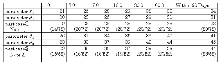
Table 5-2 Past Cases and Largest
Aftershock Occurrence Probability
(Trial Calculation)
[2] Past Cases and Largest Aftershock Occurrence Probability
When a large aftershock has occurred, it is important to evaluate if it is the largest aftershock. It is also possible to use probability expressions to represent the occurrence of the largest aftershock. Here "largest aftershock occurrence probability", is the probability R that the largest aftershock with a magnitude of M* or more occurs in the subsequent time period [T1,T2] , and R is obtained by the following equation.
R = Pr{the largest aftershock with a magnitude of M* or more occurs in the subsequent time period[T1, T2]}
= Pr{the magnitude
of the largest aftershock in the subsequent time period[0,![]() ]
is M*or more}×Pr{aftershock occurs in the subsequent
time period[T1,T2]}
]
is M*or more}×Pr{aftershock occurs in the subsequent
time period[T1,T2]}
![]() the first item
the first item ![]() the second item ('Pr{}is the probability.)
the second item ('Pr{}is the probability.)
Here ,
The first item in equation (28) is
equation (16) that substitutes for T1 = 0, T2=![]() ,
M
= M*. Using
,
M
= M*. Using ![]() in equation (26) and
in equation (26) and ![]() = b ln 10, the first item represent as:
= b ln 10, the first item represent as:
The equation (29) shows double exponential
distribution as extreme value distribution(Utsu, 196 1).
As already explained, the calculation
in a case where p![]() 1.0
must be performed by providing a sufficiently large value for
1.0
must be performed by providing a sufficiently large value for ![]() .
Table 5-2 presents past cases along with the results of trial calculations
using the trial calculation parameters
.
Table 5-2 presents past cases along with the results of trial calculations
using the trial calculation parameters ![]() and
and ![]() referred
to in [1].
referred
to in [1].
The probability of the occurrence of the largest aftershock is almost identical to the calculated probability using the average parameters in Table 5-1. But at the time that a large aftershock occurs, it is difficult to state that it is the largest aftershock.
The hypocenter parameters used for the past cases include information that is less precise than that available now, and there are some earthquakes where it is not clear if it should be considered to be an ordinary aftershock or an aftershock in the wide sense.
According to the information obtained
here, the largest aftershock of an inland earthquake often occurs within
one week (Of the 72 past cases of activity, 20 were accompanied by large
aftershocks that could cause damage, and of these, 18 occurred within 7
days), while in the sea area, the largest aftershock is a little later.
To refer to the largest aftershock, it should be as large as those cited
in the past examples.
In the past cases, the largest aftershock occurred within 30 days of an inland earthquake and almost always within 90 days after an earthquake in the sea area. But the probability based on the trial calculation parameters slightly increase as the application period lengthens. According to trial calculation parameter θ2 for example, there is an approximately 8% probability of the largest aftershock occurring between 1 year and 1 million days (about 2,700 years) after a mainshock. Probabilities over long time periods are primarily determined by K and p but it is more natural to think that this exceeds the limit to the applicability of the aftershock stochastic model.
The limit to the applicability of the aftershock stochastic model has not been uniformly determined considering the fact that the aftershock activity following the Nobi Earthquake (M8.0) of 1981 can be represented for several decades with the MO Formula. It should be considered for the time being that one month or so is appropriate for aftershock probability evaluation that can be contrasted with other models (the ETAS model for example) at the stage where the parameters can be found stably.
Inversely, looking at probability
evaluations at an early stage, the results of the trial calculations show
that the values of c and p have little effect on probability
over particularly short time periods. The value of D is closely
related to the value K from equation (21), and even the value K
alone
should, for particularly short period probability, be found before the
other parameters using the method described in part 1) (the comparison
with AIC method). One method of doing this is using data concerning the
times of felt earthquakes. It is assumed that inland, a felt earthquake
has a magnitude of at least M3. When felt earthquake information
is unusable, it is possible to use high sensitivity seismographs far from
the hypocenter to record the times of earthquakes that exceed a certain
amplitude for use as data to find the value of K.
(1) Earthquakes Whose Aftershock Probability is Evaluated
Aftershock probability evaluation is one basis for judgments made in the course of emergency measures and restoration activities conducted by residents, business offices, disaster prevention organizations, etc. in areas struck by an destructive earthquake. For this reason, aftershock probability evaluation must be carried out after any earthquake that could be followed by aftershocks capable of inflicting new damage.
Earthquakes of this kind are thought
to be those with a maximum seismic intensity more than 5 Lower: the level
where conspicuous damage begins to appear. If an earthquake of this kind
is a mainshock, it is possible that seismic intensity equal to that of
the mainshock will be locally observed, or according to circumstances,
even higher than the mainshock. For this reason, whenever an earthquake
of this kind has occurred on land or in the sea area, evaluation work has
to begin immediately without regard to its location.
Much real seismic activity follows a complex course depending on where it occurs its magnitude, and its type, so it is impossible to cover all methods of evaluating aftershock probability at the time an earthquake occurs.
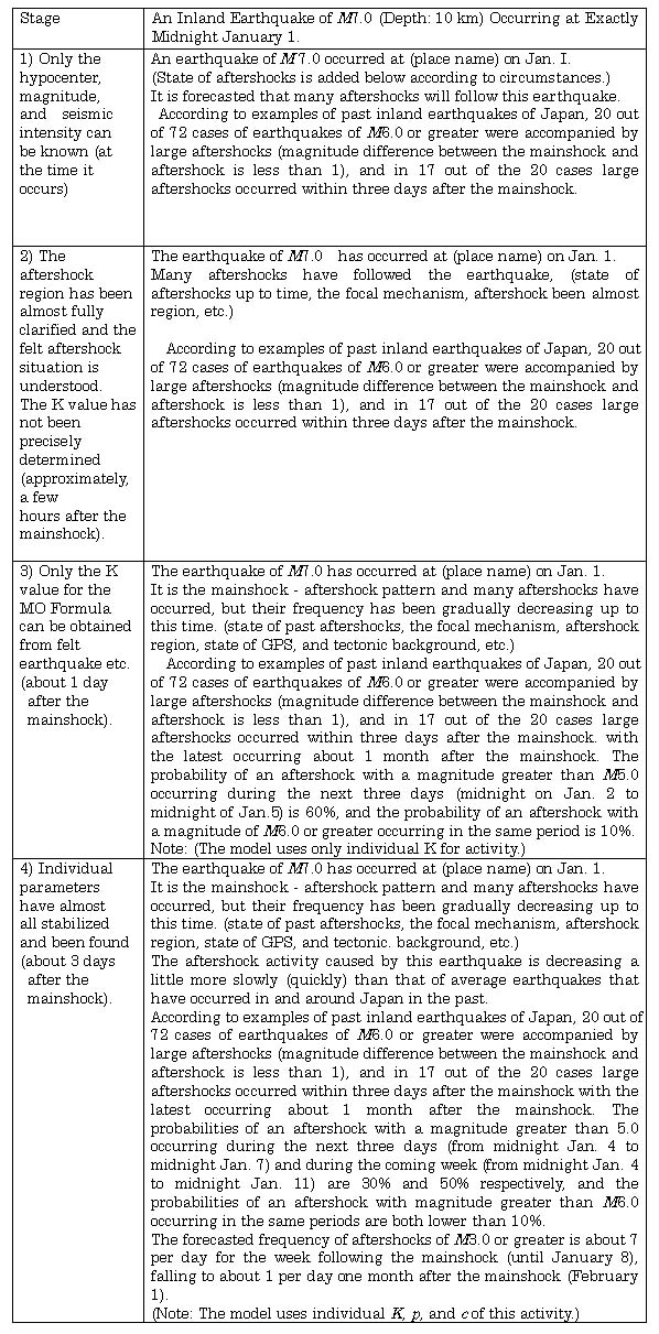
This section presents the aftershock probability evaluation method that should be implemented, the content of the evaluations of aftershocks, and examples of the representation of evaluation results at each of the hypothetical stages following a magnitude 7.0 shallow inland earthquake selected as a concrete example of common mainshock - aftershock activity.
When actually applying these methods, they have to be selected and applied flexibly and when more advanced analysis technology has become available, it must be appropriately incorporated.
Stage 1.
Hypothesis: Only the hypocenter, magnitude, and seismic intensity can be known (at the time it occurs).
Based on "2, (1) Mainshock - Aftershock Pattern Clarification", the magnitude 7.0 shallow inland earthquake is treated as the mainsbock, and it can be assumed that mainshock - aftershock activity will occur. At this stage, the aftershock activity can not be clarified, so preparation for aftershock probability evaluation (selection of observation points suitable for the monitoring, the activity of felt earthquake) is carried for the next stage.
The content of evaluation at this stage consists of past statistical cases.
Stage 2.
Hypothesis: The aftershock region has been almost fully clarified and the felt earthquake activity is understood. The K value has not been precisely determined (generally, a few hours after the mainshock).
The application of the MO Formula
began. Based on the cumulative aftershock frequency chart, it has been
confirmed whether it is represented with a single MO Formula or not. And
the process of using the time of the felt earthquakes to find the parameters
of MO Formula (average parameters (K ,![]() ,
,![]() )
and individual parameters (K, c, p)) has begun.
)
and individual parameters (K, c, p)) has begun.
The content of the evaluation at this stage are the aftershock situation and past statistical cases.
When the value of K has been
determined, it is possible to perform probability evaluation based on the
average parameters (K ,![]() ,
,![]() )
, but because is used, the evaluation should be limited to short time periods
(3 days for example).
)
, but because is used, the evaluation should be limited to short time periods
(3 days for example).
Stage 3.
Hypothesis: Only the value K for the MO formula can be obtained from felt earthquakes etc. (about 1 day after the mainshock).
It is important to compare the AIC of two models (average parameters and individual parameters) based on the work performed since stage 2.
The contents of the evaluation are
the aftershock situation and past statistic examples, along with an aftershock
probability evaluation based on the more appropriate model (here, the average
parameters (K ,![]() ,
,![]() )).
And because the value of p can not generally be relied on when there
is little data the long term probability can greately deviate. At this
stage, the evaluation should be limited to extremely short term (3 days
for example).
)).
And because the value of p can not generally be relied on when there
is little data the long term probability can greately deviate. At this
stage, the evaluation should be limited to extremely short term (3 days
for example).
Stage 4
Hypothesis: Individual parameters have almost all stabilized and been found (about 3 days after the mainshock).
At this stage, if p is stable, long term evaluation is possible and this kind of evaluation is considered to be effective information for the restoration and recovery work and others in the stricken district. In this case, it is important that the information includes forecasts of the number of aftershocks of M3.0 or greater which approximately represents felt shallow inland earthquakes.
The content of the evaluation includes revised content at Stage 3 along with relatively long term aftershock probability evaluation, aftershock frequency forecasts, etc.
Table 6 presents an example of the concrete expressions of evaluation results at Stages 1 to 4.
Table 6. presents probability rounded off to 10% units (a significant figure:
1) because this level of error is anticipated.
As shown in "1. (2) Fundamental Concepts," in addition to these types of information it is important that effective information, or in other words, the following items that are indicated in "2. Methods of Evaluating Aftershock Probability" are appropriately added according to circumstances.
- When an earthquake has occurred near an active volcano (or near a Quaternary volcano), information such as: "according to past cases, an aftershock whose magnitude is close to that of the mainshock is likely to occur in an active volcano region(or by geological effects)''.
- In the sequence occurrence regions in the sea area, information such as, "according to past cases, an earthquake of almost the same size (or aftershocks of almost same magnitude of the mainshock) is likely to occur in this sea area."
- When almost no aftershocks have been observed, this fact.
- When secondary aftershocks have been conspicuous or an earthquake larger than the mainshock has occurred, probability evaluation results based on an more appropriate model by means of a comparison between models that using applies a single MO Formula and multiple MO formulae.
Table 6. Example of Concrete Expressions
of Evaluation of an Inland Earthquake
A destructive earthquake is an event which most people experience no more than once in their lifetime. When a destructive earthquake has just occurred, earthquake information, particularly that concerning aftershock probability, is initially unfamiliar to most people, so officials in charge of taking action to deal with disasters have to understand its significance. To provide them with this knowledge, it is important to create as many opportunities as possible for them to become familiar with it. Measures must be planned and implemented enabling disaster officials to learn how to make effective use of this information through ongoing training and educational activities at normal times; not just following a destructive earthquake.
It is vital that they be given information that provides them with sufficient awareness of the methods described in the preceding sections of this rept6rt, with the premises for the use of these methods, average aspects of aftershock activities, and the significance of numerical probabilities.
It is also vital to hear the views
and needs of administrative agencies, residents, and business offices that
will receive information concerning aftershock probability evaluations,
and to consider the results of surveys conducted to forecast how these
recipients will act on the basis of the aftershock probability information
they obtain.
This study of aftershock probability evaluation methods has been conducted based on present day technology established in the field of seismology. But, earthquake observation methods, and seismological analysis technology are all advancing. In the field of earthquake activity evaluations, the ETAS model plays an extremely important role in the objective clarification of everything from mainshock - aftershock activity I to earthquake swarms, so it is necessary to continue to study ways to use the model in anticipation of ongoing research on the ETAS model based methods and in response to its results.
The methods described in this report must be the subject of further research to incorporate more precise hypocenter parameters and new cases, appropriately review the average parameters, and develop methods of estimating the individual parameters at an earlier stage.
And it is important to conduct surveys of the recipients of aftershock probability evaluations referred to in 3 (3) along with surveys of cases where aftershock probability evaluations have actually been carried out.
While outside the scope of this study, the residents were deeply concerned with the following three matters related to aftershocks. This report also refers to the explanation possible now.
[1] Time of occurrence of large aftershocks: Under present circumstances, it is difficult to conclusively forecast when a large aftershock will occur. Several reports have claimed that a large aftershock is immediately preceded by the so-called seismic quiescence, a temporary decline in aftershock activity. But there are cases where a period of seismic quiescence is not followed by a large aftershock, or cases where a large aftershock occurs without a period of seismic quiescence. It is, therefore, difficult to predict an imminent large aftershock under present circumstances, so more cases will have to be studied if this phenomena is to become a useful source of information for predictions.
[2] Location of large aftershocks: It is possible to designate the location where a large aftershock will occur at the ''close to the aftershock regions level, but it is difficult to offer anything more precise under present conditions. They often occur near the edges of aftershock regions, but exceptions to this rule are not rare. In a recent case, the largest aftershock (April 3, M5.6) following a March 26, 1997 earthquake (M6.5) in the north-western part of Kagoshima Prefecture in Japan occurred a little to the west of the epicenter distribution, but it was not in an area that could be defined as the edge of the aftershock region. Further research is necessary to abstract areas of stress concentration, parts left at the main shock rupture, and bends in the faults, etc. based on analysis of the three dimensional hypocentral distribution. The relationships characteristic of earthquakes that occur far from aftershock regions are not well understood. This type include the so-called induced earthquakes and aftershocks in the wide sense of the term: the Mikawa Earthquake (M6.8) of 1945 that followed the Tonankai Earthquake (M7.9) of 1944 for example. To obtain this knowledge, more cases have to be studied and analyses accounting for changes in stress distribution caused by the main shock have to be performed.
[3] Shaking at specified locations
caused by large aftershocks: Because conditions prevent forecasting of
locations where large aftershocks will occur, under present circumstances,
it is difficult to do so. Qualitatively, it is necessary to provide a commentary
pointing out that ''it is possible that at a certain place in the aftershock
region, a seismic intensity equal to or greater than a certain level will
occur." Because residents earnestly desire these kinds of information,
it is important to carry out future fundamental surveys and observations
to improve hypocenter determination capabilities and to study more past
cases, and in this way to contribute to the advance of research in this
field.
Abe, Katsuyuki (1991): Probability forecast of aftershocks, Zisin, 2, 44, 145 - 146.
Abe, Katsuyuki (1994): Probability forecast of aftershocks (Errata), Zisin, 2, 47,239.
Akaike, H (1974): A new look at the statistical model identification, IEEE,Trans. Autom. Contro,AC-19, 716 - 723.
Guo, Z. and Y. Ogata (1997): Statistical relations between the parameters of aftershocks in time, space, and magnitude, J. Geophys. Res., 102, 2857 - 2873.
Gutenberg, B. and C.F. Richter (1941): Seismicity of the earth, Geo1. Soc. An., Special Papers, No. 34.
Gutenberg, B. and C.F. Richter (1944): Frequency of earthquakes in California, Bull,Seism. Soc. Am., 34, 185 - 188.
Hamada, Nobuo (1990): Some amendments for the earthquake catalogue in the special issue No.6 of the Seismological Bulletin of the Japan Meteorological Agency, Zisin, 2, 43, 307 - 310.
Hoshiba, Mitsuyuki, Masaaki Seino, Masami Okada and Hidemi Ito (1993): A list of spacetime inter-relationship in earthquake occurrence and its applications, Papers in Meteology and Geophysics, 44, 83 - 90.
Hosono, Koji and Akio Yoshida (1992): Farecasting Aftershock activities, Papers in Meteology and Geophysics, 42, 145 - 155.
Isshiki, Naoki, Kazunori Matsui and Koji Ono(1968a): Volcanoes of Japan (first edition), Geological Survey of Japan.
Isshiki, Naoki, Kazunori Matsui and Koji Ono(1968b): Volcanoes of Japan (first edition), Selected Literatures on Volcanoes, Geological Survey of Japan.
Ito, Hidemi, Kazumitsu Yoshikawa, Akihiko Wakayama, Akio Yoshida,and Masaaki Seino (1999): Some empirical criteria for judging whether a shock is accompanied by a shock with larger or almost the same magnitude, submitted to Quarterly Journal Seismology. Edited by the Japan Meteorological Agency (1996): National catalogue of the active volcanoes in Japan (second edition), 500p.
Kondo, Sukehiro, Toshiro Koyanagi, Shimpei Kawauchi, Mitsuhiro Nakagawa, Sadaomi Suzuki, Sakae Hasagawa, To Yamanouchi, Momoki Kawabe, Koji Kishi and Yasuyuki okahisa (1989): Recent activity at the Maruyama Volcano in the Higashi Daisetsu Mountain System, Program and Abstracts the Volcanology Society of Japan, No. 2, 160.
Matsu'ura, R.S. (1986): Precursory quiescence and recovery of aftershock activity before some large aftershocks, Bull. Earthq. Res. Inst., University of Tokyo, 61, 1 -65.
Matsu'ura R.S. (1993): On parameter
values for the modified Omori Formula - aftershock activity of M![]() 6.0 in Japan (1969 - 1991), Abstract 1993 Japan Earth and Planetary Science
Joint Meeting, 224.
6.0 in Japan (1969 - 1991), Abstract 1993 Japan Earth and Planetary Science
Joint Meeting, 224.
Matsu'ura R.S. (1995): The centenary of the Omori formula - study of aftershock decay Zisin, 19, 33 - 34.
Nakagawa, Mitsuhiro, Hironori Maruyama and Atsushi Funayama (1995): Distribution and Spatial Variation in Major Element Chemistry of Quaternary Volcanoes in Hokkaido, Japan, Bull.Volcanological Society of Japan, 40, 13 - 31.
Ogata, Y. (1983): Estimation of parameters in the modified Omori Formula for aftershock frequencies by the maximum likelihood procedure, J. Phys. Earth, 31, 115 - 124.
Ogata, Y. (1986): Statistical models for earthquake occurrences and residual analysis for point processes, Mathematical Seismology, 1, 228 - 281, Inst. Statist. Math.
Ogata, Y. (1988): Statistical models for earthquake occurrences and residual analysis for point processes, J.Am. Stat. Assoc., 83, 9 - 27.
Ogata, Y. (1989): Statistical model for standard seismicity and detection of anomalies by residual analysis, Tectonophysics, 169, 159 - 174.
Ogata, Y. (1992): Detection of precursory relative quiescence before great earthquakes through a statistical model, J. Geophys. Res., 97, 19845 - 19871.
Ogata, Y. (1994): Seismological application of statistical methods for point- process modeling, in Proceedings of the first US/Japan conference on Frontiers of Statistical Modeling, ed. H. Bozdogan, 37 - 163, Kluwer Academic Publishers, Dordrecht.
Ogata, Y. and K. Shimazaki (1984): Transition from aftershock to normal activity, Bull. Seismol. Soc.Am., 74, 1757 - 1765.
Okada, Masami (1979): Statistical distribution of the difference in magnitude between the main shock and its largest aftershock, Zisin, 2, 32, 463 - 476
Omori, F. (1894): On the aftershocks of earthquakes, J. Coll. Sci. Imp. Univ. Tokyo, 7, 111-200.
Omori, F. (1894): On aftershocks, Report by the Earthquake Investigation Committee, 2, 103 - 139, in Japanese.
Ohtani, Tomo, Tatsuo Sekiguchi, Kazumasa Haraguchi (1993): Development of the volcanic landform data-base, Programme and Abstracts the Volcanological Society of Japan, No. 2, 30.
Ono, Koji, Tatsunori Soya, Koji Mimura (1981): Volcanoes of Japan (second edition), Geological Survey of Japan.
Reasenberg, P.A. and L.M. Jones (1989): Earthquake hazard after a mainshock in California, Science, 243, 1173 - 1176.
Reasenberg P.A. and L.M. Jones (1994): Earthquake aftershocks: update, Science, 265, 1251 - 1252.
Seino, Masaaki, Akio Yoshida and Toshikazu Odaka (1995): On the relations between the occurrence of inland earthquakes and the volcanic regions, Abstracts 1995 Japan Earth and Planetary Science Joint Meeting, 291.
Seismic Countermeasures Section, Shizuoka Prefecture (1993): Basic study of the characteristics of and countermeasures to deal with aftershock activity following the occurrence of a Tokai Earthquake, 135 p.
Prime Minister's Office (1995): Public opinion survey concerning earthquakes, 33 p.
Utsu, T. (1961): A statistical study of the occurrence of aftershocks, Geophys. Mag., 30, 521-605.
Utsu, T. (1969): Aftershocks and earthquake statistics (1), J. Fac. Sci., Hokkaido Univ., Ser. 7, 2, 129- 195.
Utsu, T. (1970): Aftershocks and earthquake statistics (2), J. Fac. Sci., Hokkaido Univ., Ser. 7, 3, 197 - 266.
Utsu, T. (1957): Magnitudes of earthquakes and occurrence of their aftershocks, Zisin, 2, 10,35 - 45.
Utsu, T. (1964): Magnitude distribution of earthquakes with special consideration to aftershock activities, Quarterly Journal of Seismology, 28, 129 - 136.
Utsu, T. (1969): Some problems of
the distribution of earthquakes in time (part 1) - distributions of frequency
and time interval of earthquakes, Geophys. Bull.
Hokkaido Univ., 22, 73 -
94.
Utsu, T. (1969): Some problems of the distribution of earthquakes in time(part 2) - stationarity and randomness of earthquake occurrence, Geophys. Bull. Hokkaido Univ.J., 22, 95 - 108.
Utsu T., Y. Ogata and R.S. Matsu'ura
(1995): The centenary of the Omori formula for a decay law of aftershock
activity,
J. Phys. Earth, 43, 1 - 33.